18 Cluster Analysis
18.1 What is ‘cluster analysis’?
Cluster analysis is a statistical technique that’s used to group similar objects into categories or ‘clusters’.
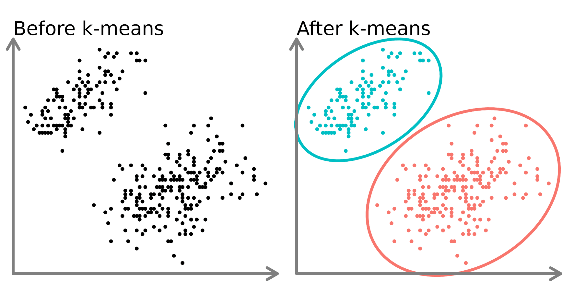
In the following figure, a dataset (left) has been ‘clustered’ into three groups (right) whose members are more similar to each other.
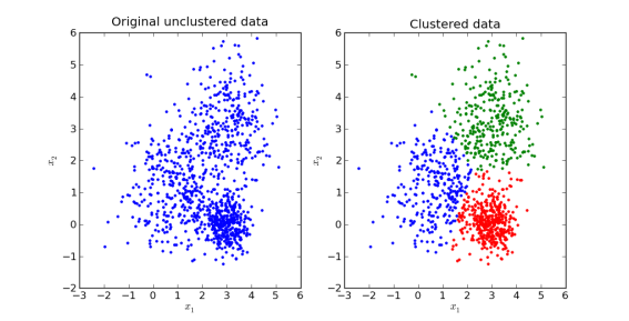
Therefore, cluster analysis identifies patterns in our data by organising it into subsets that share common characteristics.
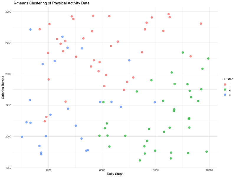
Imagine a diverse group of individuals engaging in a physical activity intervention. You collect data on their daily steps, their active minutes per day, and their calories burned per day.
By conducting a cluster analysis, you could ‘group’ the individuals into three clusters or ‘types’, for example Cluster One (red - higher calories burned with a range of daily steps), Cluster Two (green - higher daily steps but moderate calories burned) and Cluster Three (blue - lower daily steps and lower calories burned).
This is really useful, because it helps us start to identify different ‘types’ of responses on multiple variables, or different groups within our data. This might in turn lead to some further research questions or analysis on those clusters.
18.2 Types of clustering
There are a number of different types of clustering you might encounter. The two most common are:
Hierarchical clustering, which builds a hierarchy of clusters either by successively merging smaller clusters into larger ones (agglomerative), or by splitting larger clusters (divisive).
Partitioning methods, which partition (divide) the dataset into a predefined number of clusters, optimising a criterion like the distance between points in a cluster.
18.3 ‘Distance’ and ‘similarity measures’
Before we explore these two types of clustering in more detail, it’s important to cover a few underpinning concepts and ideas in cluster analysis.
Cluster Analysis involves examining the distance between and similarity to data points in order to build clusters.
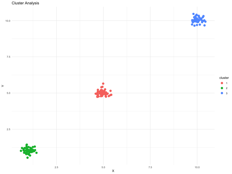
Here is an (artificial) example of a cluster analysis which minimises intra-cluster distance, and maximises inter-cluster distance:
We can use a number of different measures of distance:
Euclidean distance is a basic metric in geometry, often used in data analysis and machine learning to measure the straight-line distance between two points in Euclidean space. It’s calculated as the square root of the sum of the squared differences between corresponding elements of two vectors.
Manhattan distance (sometimes called the L1 norm or “city block” distance) measures the sum of the absolute differences between points in a grid-like path. Unlike Euclidean distance, it calculates the total distance traveled along axes at right angles, mimicking how one would navigate a city’s grid-like streets.
Cosine similarity is a measure used to determine the cosine of the angle between two non-zero vectors in an inner product space. This metric evaluates the similarity irrespective of their size, focusing on the orientation rather than the magnitude of the vectors.
The Jaccard Index (or Jaccard similarity coefficient) is a statistic used for gauging the similarity and diversity of sample sets. It measures similarity as the size of the intersection divided by the size of the union of the sample sets.
Imagine you’re standing at one corner of a football field, and your friend is at another corner. You could walk along the edges of the field to reach your friend, but that would be a longer way.
The quickest way is to walk directly from your corner to your friend’s corner, cutting across the field. This straight line you walk is the shortest distance between you two, and that’s what’s called ‘Euclidean distance’.
In maths, we use this idea to measure the straight-line distance between two points in space, no matter how many dimensions that space has. It’s like using a ruler to measure the distance between two dots on a piece of paper, but it also works for spaces that have more than two dimensions, which is a bit harder to imagine but works on the same principle.
18.4 Criteria for good clustering
‘Intra-cluster’ and ‘inter-cluster’ distances
The major objective for effective clustering is to optimise the intra-cluster (small as possible) and inter-cluster (big as possible) distances.
Intra-cluster distance is the compactness of the clusters, meaning how close the data points within the same cluster are to each other. Ideally, a good cluster has a small intra-cluster distance, indicating homogeneity within the cluster.
Inter-cluster distance is the separation between different clusters. Effective clustering ensures that the inter-cluster distance is maximised, giving clear differentiation between clusters.
Balancing these two aspects is crucial for creating distinct, meaningful clusters that accurately reflect the underlying structure of the data.
Cluster validity indices
Cluster validity indices are quantitative measures used to evaluate the goodness of a clustering structure. These indices help us determine the optimal number of clusters and assessing the quality of the clusters formed.
Common indices include the Davies-Bouldin index, Silhouette index, and the Dunn index.
The Davies-Bouldin index, for instance, is based on a ratio of intra-cluster to inter-cluster distances, with lower values indicating better clustering.
18.5 Type One: Hierarchical clustering
Now, let’s look at some common forms of cluster anaysis.
Hierarchical clustering is a method of cluster analysis which seeks to build a hierarchy of clusters. It’s widely used in fields like data mining, statistics, and machine learning.
Algorithm overview
We can approach the computational aspect of hierarchical clustering in two ways:
‘Agglomerative’ is a “bottom-up” approach. Initially, each data point is considered as a separate cluster. Then, pairs of clusters are merged as one moves up the hierarchy.
The process continues iteratively until all points are merged into a single cluster or until a desired structure is achieved. Common linkage methods (criteria for choosing the cluster pair to merge) include minimum, maximum, average, and Ward’s linkage.
‘Divisive’ is a “top-down” approach. It starts with all data points in a single cluster and iteratively splits the cluster into smaller clusters. At each level, the cluster to split is chosen, and it is divided into two least similar parts.
This method is less common and more computationally intensive than agglomerative.
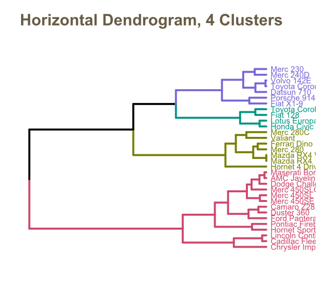
Dendrograms
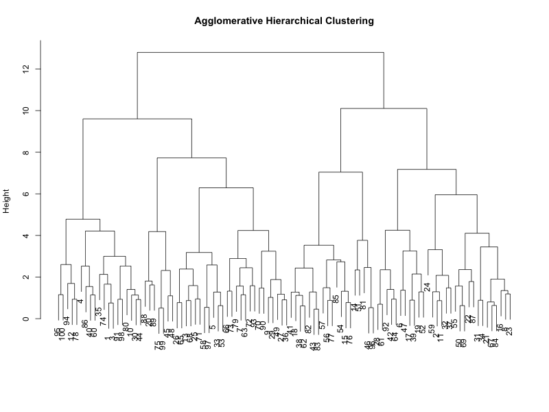
A dendrogram, like the figures above, is a tree-like diagram that records the sequences of merges or splits from a hierarchical clustering approach.
The vertical lines represent the clusters being merged (in agglomerative) or split (in divisive), and their height indicates the distance or dissimilarity between clusters.
Shorter vertical lines indicate similar clusters. By cutting the dendrogram at a specific height, you can determine the number of clusters. This “cut-off” point is subjective and can significantly affect the results.
18.6 Type Two: Partitioning methods
Hierarchical methods seek to separate observations into smaller and smaller groups, or clusters.
Partitioning methods, on the other hand, are techniques that divide data sets into distinct subsets or clusters. We’ll focus on two methods: K-means clustering and K-medoids.
K-means clustering
K-means clustering is used in data analysis to group similar items together.
Imagine you’re a PE teacher responsible for organising a school sports day (lucky you!).
You have a large group of pupils and you want to divide them into different teams for a variety of games.
Each pupil has different athletic abilities, like running speed, jumping height, and throwing distance. Your goal is to create teams that are balanced and competitive.
Here’s how K-means clustering would work in this scenario:
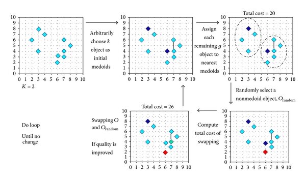
Deciding the number of teams: First, you decide on the number of teams you want to create. This is like choosing the number of clusters in K-means clustering.
Initial team captains (centroids): You randomly select a few pupils to be the initial team captains. These captains are like the initial centroids in K-means clustering.
Assigning pupils to teams: Each pupil is assigned to the team of the captain they are most similar to in terms of athletic abilities. This is like assigning data points to the nearest cluster centroid.
Re-evaluating your team captains: After all pupils are assigned, you review each team’s overall athletic ability and select a new captain who best represents the team’s average ability. This step is akin to recalculating the centroid of each cluster in K-means.
Repeating the process: You reassign pupils to teams based on the new captains, and then select new captains again. This process is repeated several times. Each time, pupils might switch teams, and new captains are chosen, aiming to create the most balanced teams possible.
Final teams: The process stops when the teams are well-balanced, and pupils’ reassignments become minimal. This means each team has a mix of pupils with varied athletic abilities, and they are as evenly matched as possible.
K-means clustering is useful because it’s a straightforward way to organise large sets of data into understandable groups based on their characteristics.
You may be wondering how we decide on the optimum number of clusters.
The ‘Elbow Method’ is a heuristic used in determining the number of clusters in K-means clustering. It involves running the algorithm for a range of ‘k’ values and plotting the total within-cluster sum of square (WSS). As ‘k’ increases, WSS tends to decrease as the data points are closer to the centroids they are assigned to.
The “elbow” point, where the rate of decrease sharply changes, represents an appropriate number of clusters. This point is chosen because adding another cluster doesn’t give much better modeling of the data.
K-medoids clustering
K-medoids is another partitioning technique. The primary difference to K-means is that K-medoids chooses actual data points as centers (medoids) rather than the mean of the data points in a cluster.
K-medoids is more robust to noise and outliers compared to K-means because medoids are less influenced by extreme values.
It is also useful because it uses actual data points as centers, and therefore can be more interpretable, especially when centroids (mean values) are not representative or meaningful.
It is also more flexible; it can work with a variety of distance metrics, not just Euclidean, making it versatile for different types of data.
18.7 Evaluating cluster quality
Evaluating the quality of clusters is important. There are various metrics we can use for evaluating cluster quality, including ‘internal’ and ‘external’ evaluation metrics.
Internal evaluation metrics
Internal metrics evaluate the quality of a clustering structure without reference to external data. They are based on the intrinsic properties of the data.
The Silhouette Coefficient is a measure of how similar an object is to its own cluster compared to other clusters. The value ranges from -1 to 1, where a high value indicates that the object is well matched to its own cluster and poorly matched to neighboring clusters.
Values near +1 indicate that the sample is far away from the neighboring clusters.
A value of 0 indicates that the sample is on or very close to the decision boundary between two neighboring clusters.
Negative values indicate that those samples might have been assigned to the wrong cluster.
The Davies-Bouldin Index (DBI) is another metric for evaluating clustering algorithms. Lower DBI values indicate better clustering.
External evaluation metrics
External metrics use external information, such as ground truth labels, to evaluate the quality of the clustering.
The Adjusted Rand Index is a measure of the similarity between two data clusterings. It is adjusted for chance, which makes it more reliable for comparing clusterings of different sizes and numbers.
ARI close to +1 indicates perfect agreement between the clusters and the ground truth.
ARI close to 0 indicates random labeling, independent of the ground truth.
Negative values generally indicate independent labelings or possibly systematic disagreement.
Normalised Mutual Information (NMI) is a normalisation of the Mutual Information (MI) score to scale the results between 0 (no mutual information) and 1 (perfect correlation).
Values close to 1 indicate a high degree of similarity between the two clusterings.
Values close to 0 indicate little or no correlation.
18.8 Challenges in clustering
High ‘dimensionality’
Clustering in high-dimensional spaces presents significant challenges. As the number of dimensions increases, the distance between data points becomes less meaningful – a phenomenon known as the “curse of dimensionality.” This makes it difficult to distinguish between clusters, as traditional distance measures lose their effectiveness.
High dimensionality also leads to increased computational complexity and the risk of overfitting, where the model captures noise rather than the underlying pattern.
Dimensionality reduction techniques like Principal Component Analysis (similar to factor analysis) are often employed to mitigate these issues, but selecting the right method and determining the optimal number of dimensions can be challenging.
Noise and outlier sensitivity
Many clustering algorithms are sensitive to noise and outliers in the data.
Noise refers to random or irrelevant data points that do not belong to any cluster, while outliers are extreme values that differ significantly from other observations.
These can significantly skew the results of clustering, leading to misinterpretation of the data or the formation of clusters that do not accurately represent the underlying structure.
Robust clustering techniques that can identify and mitigate the impact of noise and outliers are essential for obtaining reliable results, but developing and implementing these techniques can be complex.
Scalability and computational complexity
Scalability and computational complexity are major challenges in clustering, especially with the ever-increasing size of datasets.
Many traditional clustering algorithms, like K-means or hierarchical clustering, can become prohibitively expensive in terms of computation and memory requirements as the dataset grows. This limits their practicality for large-scale applications.
Developing algorithms that can efficiently handle large volumes of data without a significant trade-off in accuracy or computational resources is very challenging (and a current ‘hot topic’).
Techniques like parallel processing, efficient data structures, and approximation algorithms are often explored to address these scalability challenges.
18.9 Further reading
https://fcbusiness.co.uk/news/data-science-for-football-business-clustering-analysis/